Introduction

In Part 1, I focused on evaluating the quality of the Formula Student bodywork using CATIA Surface Analysis. By examining surface continuity, curvature, and reflection behavior, I identified the areas that required closer attention before moving into CFD. With the geometry validated, I continued with a SIMULIA CFD analysis to investigate how the bodywork interacts with airflow and prepare the model for aerodynamic evaluation.

In this article, I will share the workflow I followed in SIMULIA Fluid Dynamics Engineer, from healing the imported geometry and creating the external fluid domain to defining the physics, generating the mesh, and interpreting the first CFD results.

This study represents a baseline aerodynamic investigation rather than a final vehicle validation. My objective was to understand the airflow behavior around the bodywork, evaluate whether the surface characteristics identified during CATIA analysis influenced the flow, and identify potential areas for future design improvements.

Moving from CATIA to SIMULIA: Planning the CFD Strategy

After completing the geometry validation and healing operations in CATIA, I transferred the model into SIMULIA Fluid Model Creation.

Having previously worked with ANSYS Fluent, I found one of the most interesting parts of this project was comparing the two CFD workflows. I noticed that the main difference was not the physics behind the simulation, but rather how each platform organizes the complete simulation process.

Comparing ANSYS Fluent and SIMULIA CFD Workflows

From my experience, ANSYS Fluent provides a very solver-focused workflow. It gives users direct access to many detailed settings, including meshing controls, discretization schemes, pressure–velocity coupling methods, turbulence models, and convergence parameters.

SIMULIA Fluid Dynamics Engineer follows a more integrated CAD-to-CFD approach inside the 3DEXPERIENCE platform. Geometry preparation, external fluid-domain creation, hex-dominant meshing, prism-layer generation, physics definition, and post-processing remain connected to the same product data environment.

Both workflows are based on finite-volume CFD methods and can be used for RANS simulations. The main difference I noticed was therefore not the equations behind the simulation, but the way the engineer interacts with the entire process.

Defining the CFD Strategy for the Baseline Study

For this first aerodynamic study, I also had to consider the limitations of a student license and the available cell-count budget. Instead of applying a very fine mesh everywhere, I focused the available elements on the regions where they would provide the most value:

• The nose region, where strong pressure gradients develop
• Surface transitions, where flow acceleration or separation may occur
• Near-wall areas, where boundary-layer behavior must be captured
• The wake region behind the bodywork

The far-field region was kept relatively coarse to save computational resources.

For the boundary layer, I planned to use body-fitted prism layers. The first-layer height, growth rate, and total thickness needed to be selected according to the turbulence model and the targeted y+ range. SIMULIA Fluid Dynamics Engineer provides this type of body-fitted meshing approach to better capture complex surfaces and near-wall flow behavior.

For the initial simulation, I selected a steady incompressible RANS approach. Since this was a baseline study, my objective was not to achieve final aerodynamic certification values, but rather to understand the main flow structures around the bodywork.

During the solution process, I monitored not only residual convergence but also aerodynamic force stability, pressure distribution, and wake development. A simulation cannot be considered reliable simply because residual values decrease; the aerodynamic forces must also reach a stable behavior.

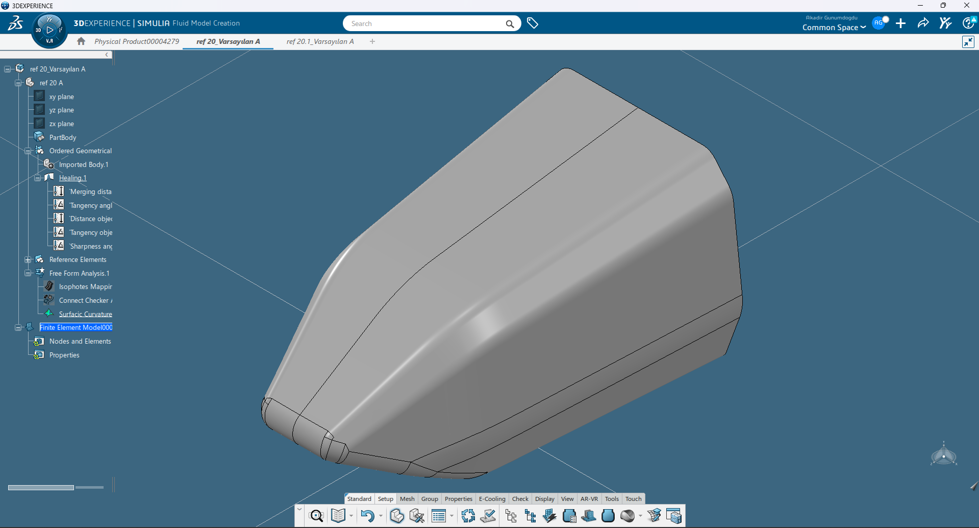
Figure 10. The healed bodywork geometry transferred to SIMULIA Fluid Model Creation before external-domain extraction and mesh generation.

Creating the External Fluid Domain

The next step was creating the external fluid domain around the bodywork using the Fluid Domain command.

This domain represents the volume of air that will be solved during the CFD analysis. Its size and the position of the vehicle inside it directly influence both the accuracy of the results and the computational cost.

When positioning the bodywork inside the domain, I maintained the intended vehicle ride height by keeping the lower boundary at the correct ground clearance.

This detail is important because the distance between the bodywork and the ground affects underbody flow, pressure distribution, and the way air interacts with the front section of the vehicle.

I also provided enough space around the vehicle to reduce artificial blockage effects. The upstream region was extended to allow the incoming flow to develop properly, while additional downstream space was reserved for wake development.

However, because I was working with a limited student-license mesh budget, I had to find a balance. A larger domain does not automatically mean better results if the additional cells are not improving the important flow regions.

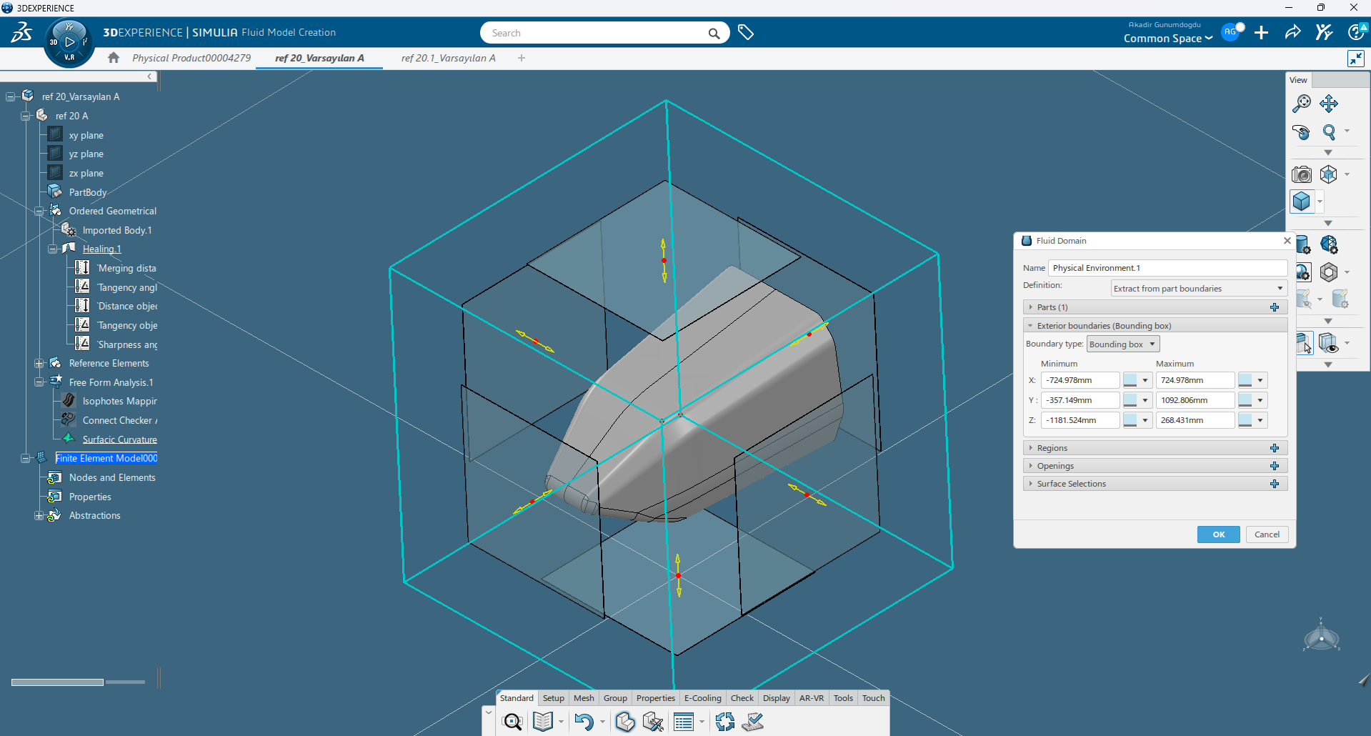
Figure 11. External fluid domain created around the bodywork.

Defining the Bodywork Region

After creating the external domain, I defined the bodywork surfaces as a separate region inside the fluid model.

This step allows SIMULIA to distinguish between the vehicle geometry and the surrounding air volume, making it possible to apply the correct wall boundary condition during the simulation setup.

At this stage, I verified that the selected faces correctly represented the bodywork and confirmed that SIMULIA could create the fluid volume without open boundaries or intersecting surfaces.

This was also an important confirmation that the geometry-cleaning process performed earlier in CATIA had successfully prepared the model for CFD.

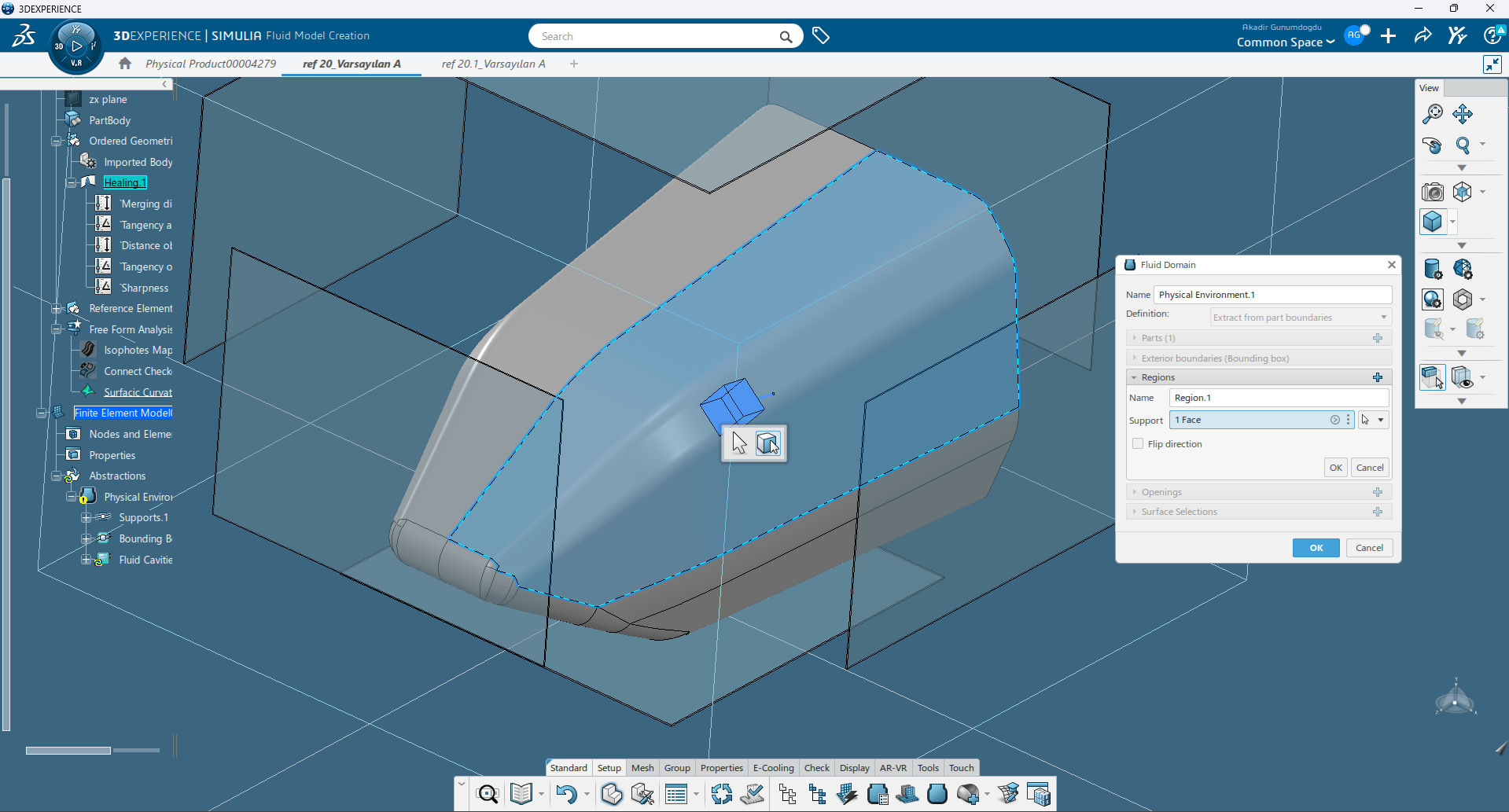
Figure 12. Bodywork surfaces defined as the fluid model region.

Physics Setup, Boundary Conditions and Output Requests

With the fluid domain prepared, I created a steady-state simulation step for the baseline aerodynamic analysis.

I set the maximum number of iterations to 2000 and defined convergence criteria for the momentum, turbulent kinetic energy (TKE), and omega equations.

These residual values provide useful information about numerical convergence, but I did not rely on them alone. I also monitored aerodynamic forces and pressure behavior to determine whether the solution had reached a physically stable state.

A simulation with low residuals can still require additional iterations if drag, lift, or pressure values continue changing.

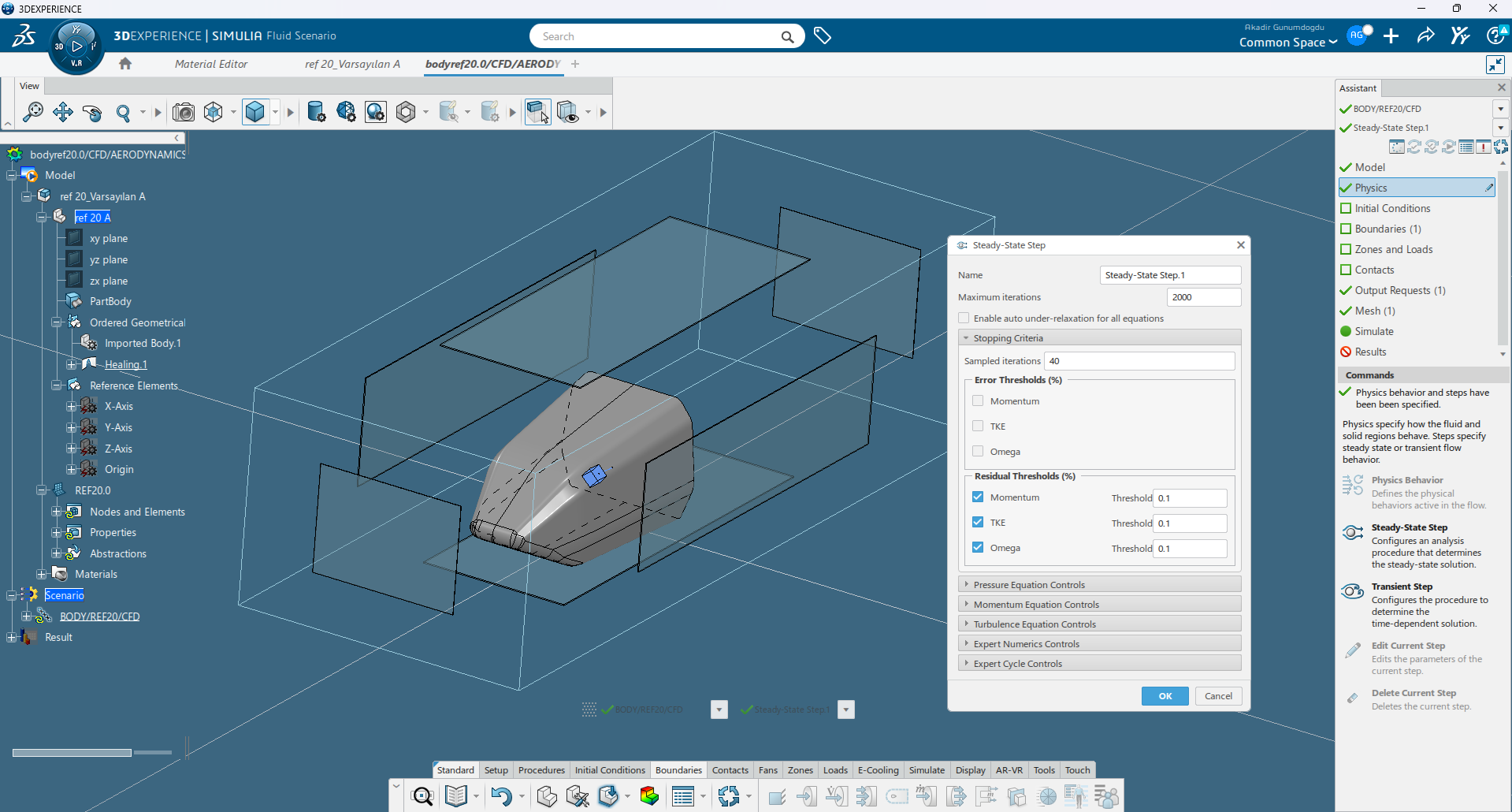
Figure 13 – Steady-state solution step with a maximum of 2000 iterations and residual stopping criteria for momentum, TKE, and omega.

Defining Boundary Conditions

For the inlet boundary, I applied a velocity inlet normal to the upstream face with a velocity magnitude of 15 m/s.

The turbulence conditions were defined using turbulence intensity and turbulent viscosity ratio, with values of 0.1 and 100 for this baseline model.

At the outlet, I applied a pressure outlet condition with a static gauge pressure of 0 Pa, allowing the flow variables to naturally develop while maintaining a reference pressure.

The bodywork surfaces were defined as solid wall boundaries. This allowed the simulation to capture important aerodynamic phenomena such as:

• Pressure accumulation around the nose
• Flow acceleration over curved surfaces
• Near-wall shear behavior
• Wake formation behind the vehicle

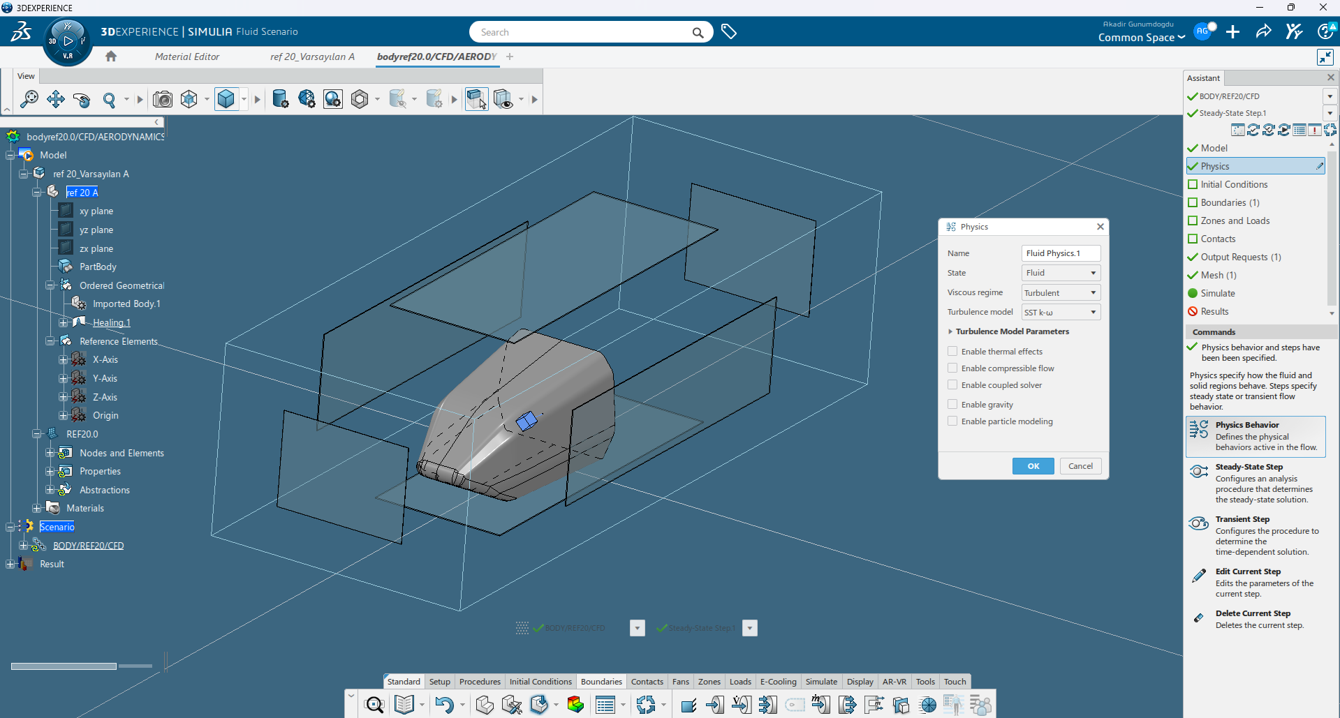
Figure 14A – Physics Behavior

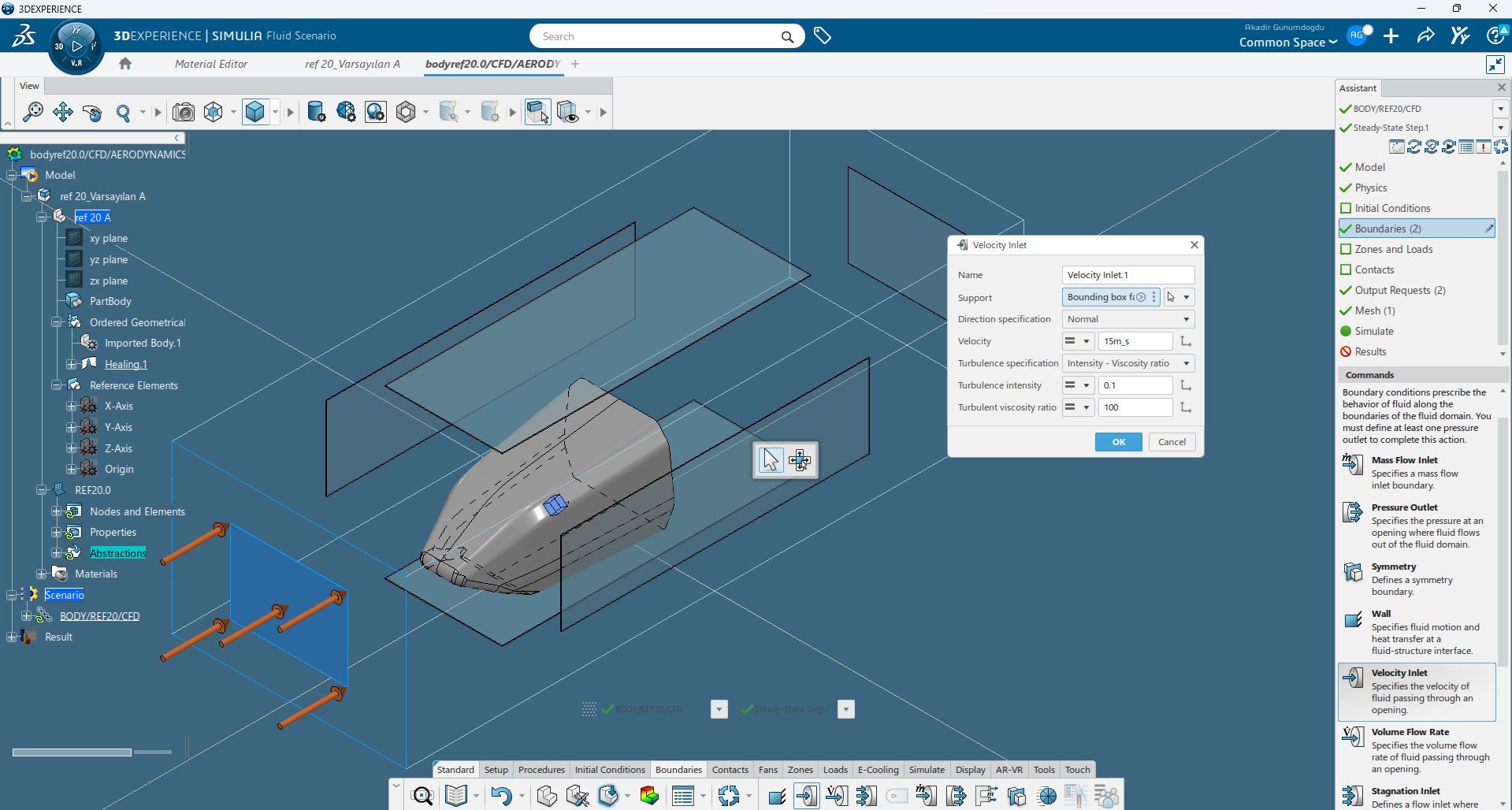
Figure 14B – Velocity inlet boundary condition applied to the upstream face with a freestream velocity of 15 m/s.

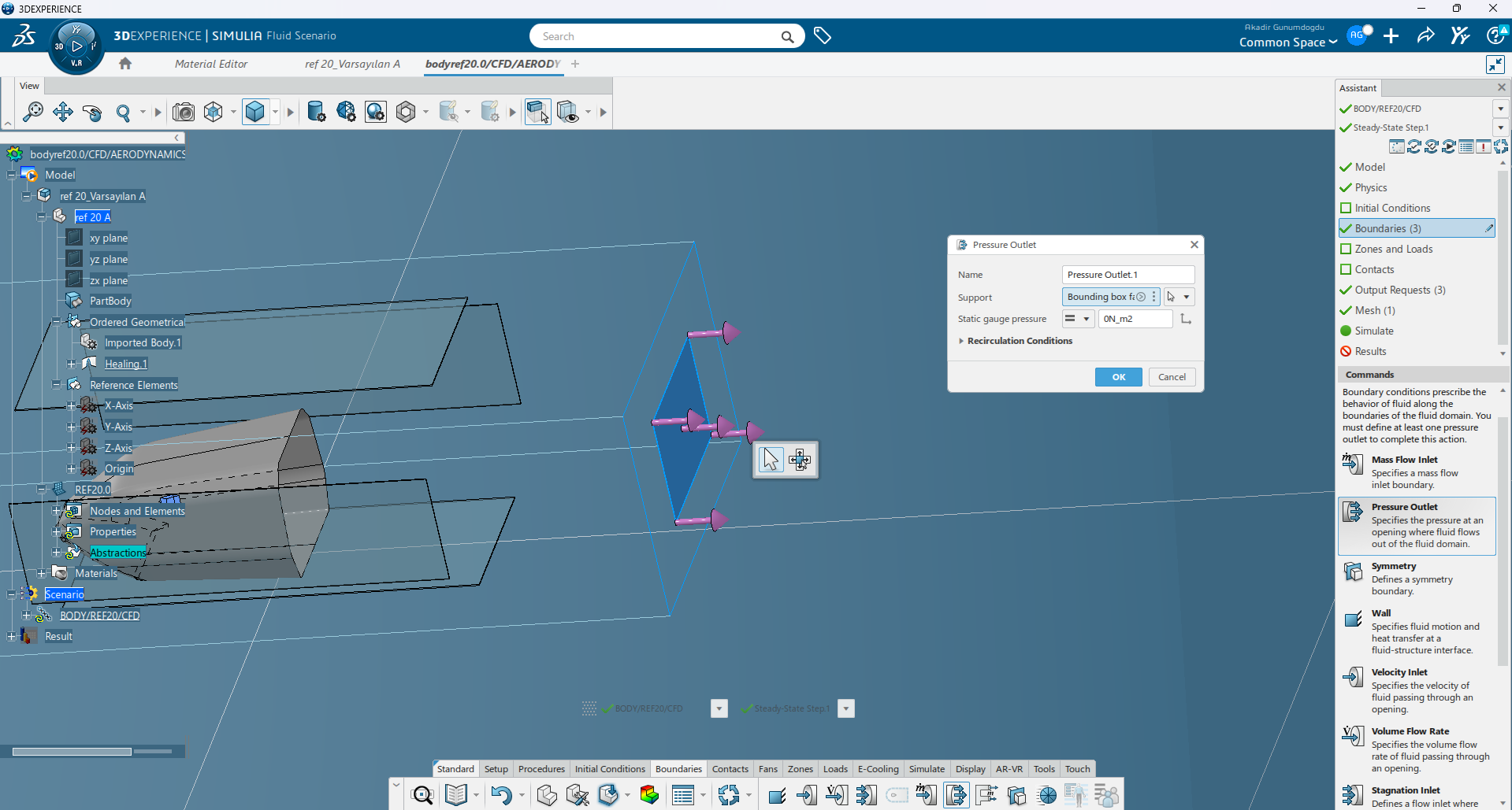
Figure 15. Pressure outlet applied to the downstream face with a static gauge pressure of 0 Pa.

Defining Field and History Outputs

Before launching the simulation, I defined both field outputs and history outputs.

Field outputs were used to visualize flow variables throughout the computational domain. The selected variables included:

• Velocity
• Gauge and absolute pressure
• Total pressure
• Vorticity
• Q-criterion
• Shear rate

These results would later help identify pressure variations, acceleration zones, rotational flow structures, and possible separation regions.

For the bodywork surfaces, I created history outputs to monitor:

• Total fluid force
• Pressure force
• Viscous force
• Moment

Tracking these values during the solution provided a clearer picture of aerodynamic convergence compared with relying only on residual plots.

I also requested wall shear and y+ values to evaluate whether the near-wall mesh was appropriate for the selected turbulence treatment.

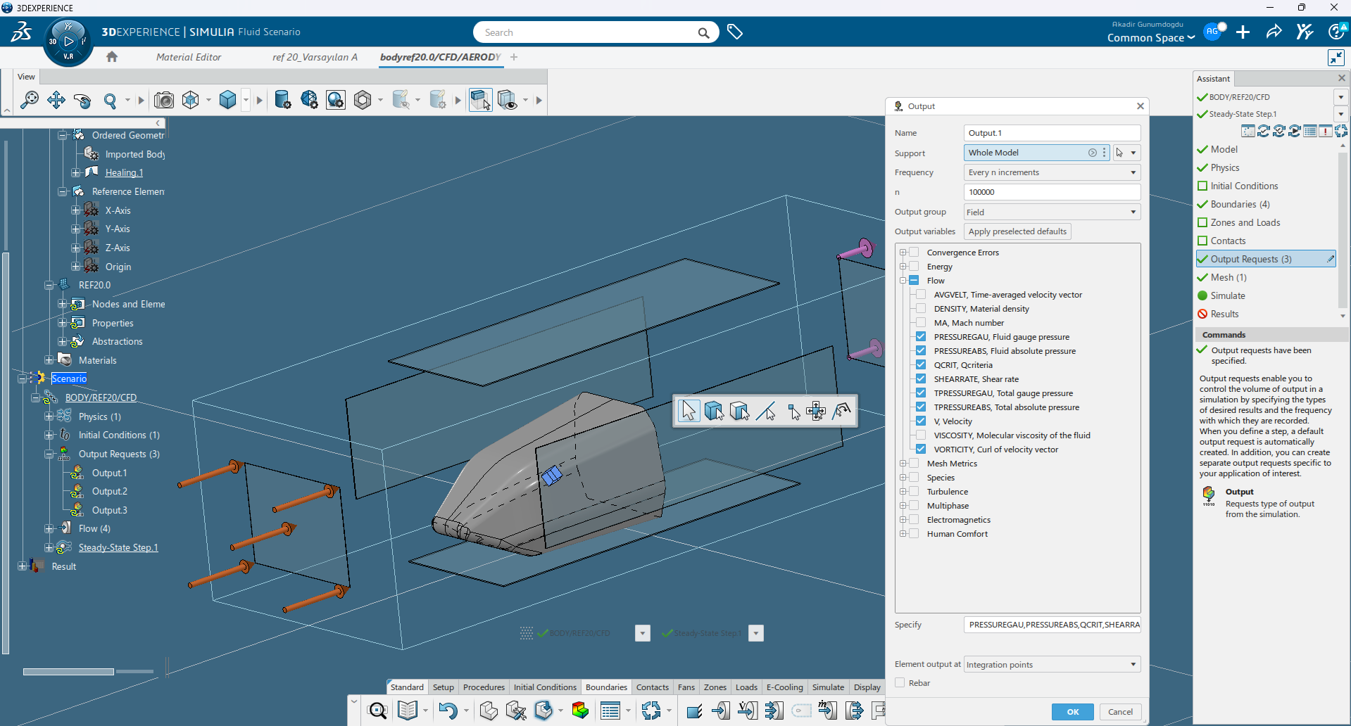
Figure 16. Output.

Hex-Dominant Mesh Strategy and Quality Check

For this baseline study, I generated a Hex-Dominant Mesh for the complete external fluid domain.

The global element size was defined between 1 mm and 5 mm, with smaller elements concentrated where more geometric detail was required. I also enabled boundary layers using seven prism layers, with a first-layer thickness of 0.2 mm.

These layers were important for capturing the velocity gradients close to the bodywork surface and for allowing the evaluation of wall shear stress and y+ values after the simulation.

However, because I was working with the limitations of a student license and a restricted cell-count budget, the mesh had to be a balance between accuracy and computational cost. For this reason, I considered this mesh as a baseline configuration rather than a final mesh-independent solution.

After mesh generation, I reviewed the quality report using several criteria, including aspect ratio, distortion, maximum and minimum angles, skewness and stretch.

The majority of the elements were within acceptable limits. A small percentage of cells were classified as poor or bad, mainly according to the aspect-ratio criterion. This was not unexpected for a complex external-flow model, where maintaining perfect element quality throughout the entire domain can significantly increase the computational cost.

The quality report confirmed that the mesh was suitable for an initial aerodynamic investigation, but it did not demonstrate mesh independence.

For a future iteration, I would avoid refining the entire domain uniformly and instead focus additional elements on the most important aerodynamic regions:

• The nose area, where pressure gradients are stronger
• Sharp surface transitions identified during CATIA analysis
• The near-wall region
• The downstream wake

This approach would provide better accuracy where it matters most while keeping the simulation cost manageable.

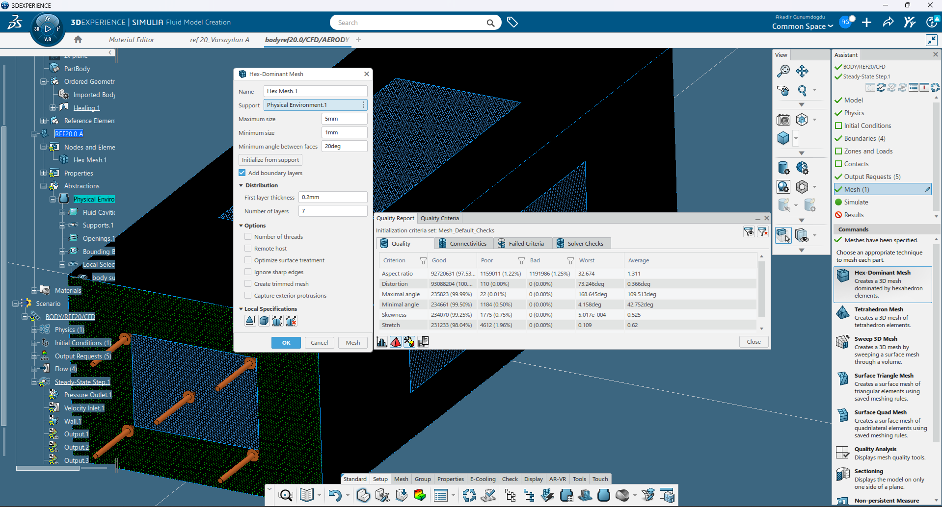
Figure 17. Hex-Dominant mesh settings and quality report for the baseline model.

Starting the Steady-State Solution and Monitoring Convergence

Once the mesh and simulation setup were completed, I launched the steady-state solution and began monitoring the results.

During the calculation, I used the history outputs to follow the evolution of the aerodynamic force components. This helped me understand whether the solution was moving towards a stable condition as the iterations progressed.

I captured the image below at approximately 1% of the simulation progress. Since the solution was still developing, the displayed force value does not represent the final aerodynamic result.

For the complete convergence assessment, I considered multiple indicators together:

• Residual behaviour of the momentum, TKE and omega equations
• Stability of the monitored aerodynamic forces
• Consistency of the pressure and velocity fields

This was an important point during the study because residual reduction alone does not guarantee that the engineering quantities have reached a stable solution.

A CFD result becomes meaningful when both the numerical convergence and the physical behaviour of the flow show a consistent trend.

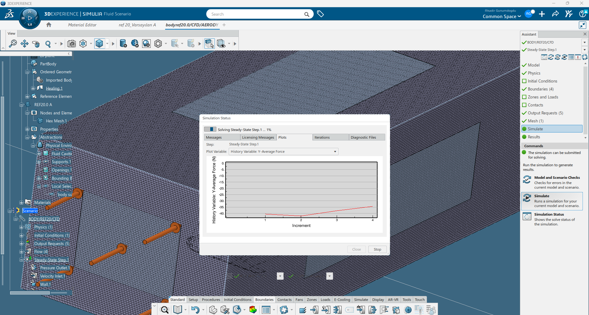
Figure 18. Initial stage of the steady-state solution with force monitoring enabled.

CFD Results and Initial Engineering Interpretation

After completing the simulation, I analysed the results by combining several visualisations, including gauge pressure contours, velocity distribution, velocity vectors and mean-flow streamlines.

Rather than relying on a single plot, I used these different results together to understand how the airflow interacted with the bodywork.

A clear stagnation region appeared at the front of the nose, where the incoming air slowed down and created a higher-pressure zone. From this point, the flow separated around the upper, side and lower surfaces of the bodywork.

As the airflow followed the curved surfaces, the velocity increased in several regions, creating lower-pressure areas. The strongest pressure variations appeared around the nose and the lower-front transition areas. The streamline and velocity-vector results also showed that the surface transitions identified during the CATIA analysis influenced the airflow behaviour.

Most of the front section maintained relatively organised flow behaviour, but downstream regions showed increasing disturbances, lower-velocity areas and wake development. The nose, lower-front corner and rear transition appeared to be the most sensitive areas of the design.

Identifying Design Limitations and Improvement Areas

These observations were consistent with the concerns identified during the Zebra, Porcupine and Surfacic Curvature analyses. However, it is important to clarify that a visible surface irregularity does not automatically mean a measurable aerodynamic penalty.

To quantify the real impact of these regions, a comparison with modified geometry and a mesh-independence study would be required.

Because this was a simplified bodywork-only CFD model, I used these results mainly to identify flow behaviour and possible improvement areas.

Limitations of the Baseline CFD Study

The simulation did not include:

• Front wing effects
• Rotating wheels
• Suspension components
• Complete vehicle aerodynamic interactions

Therefore, these results should not be considered the final aerodynamic performance of the Formula Student vehicle, but rather a first step toward understanding and improving the design.

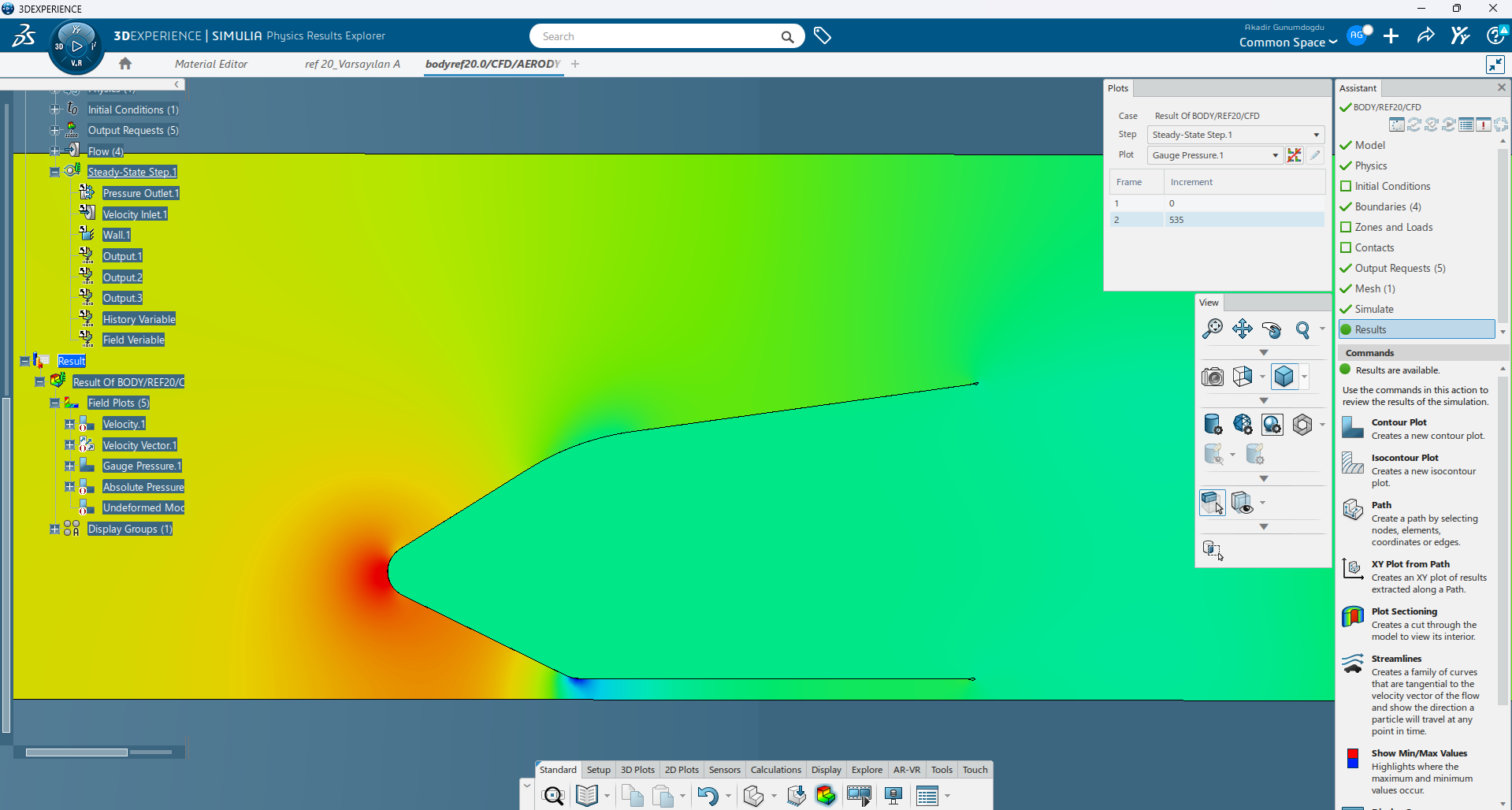
Figure 19. Gauge Pressure

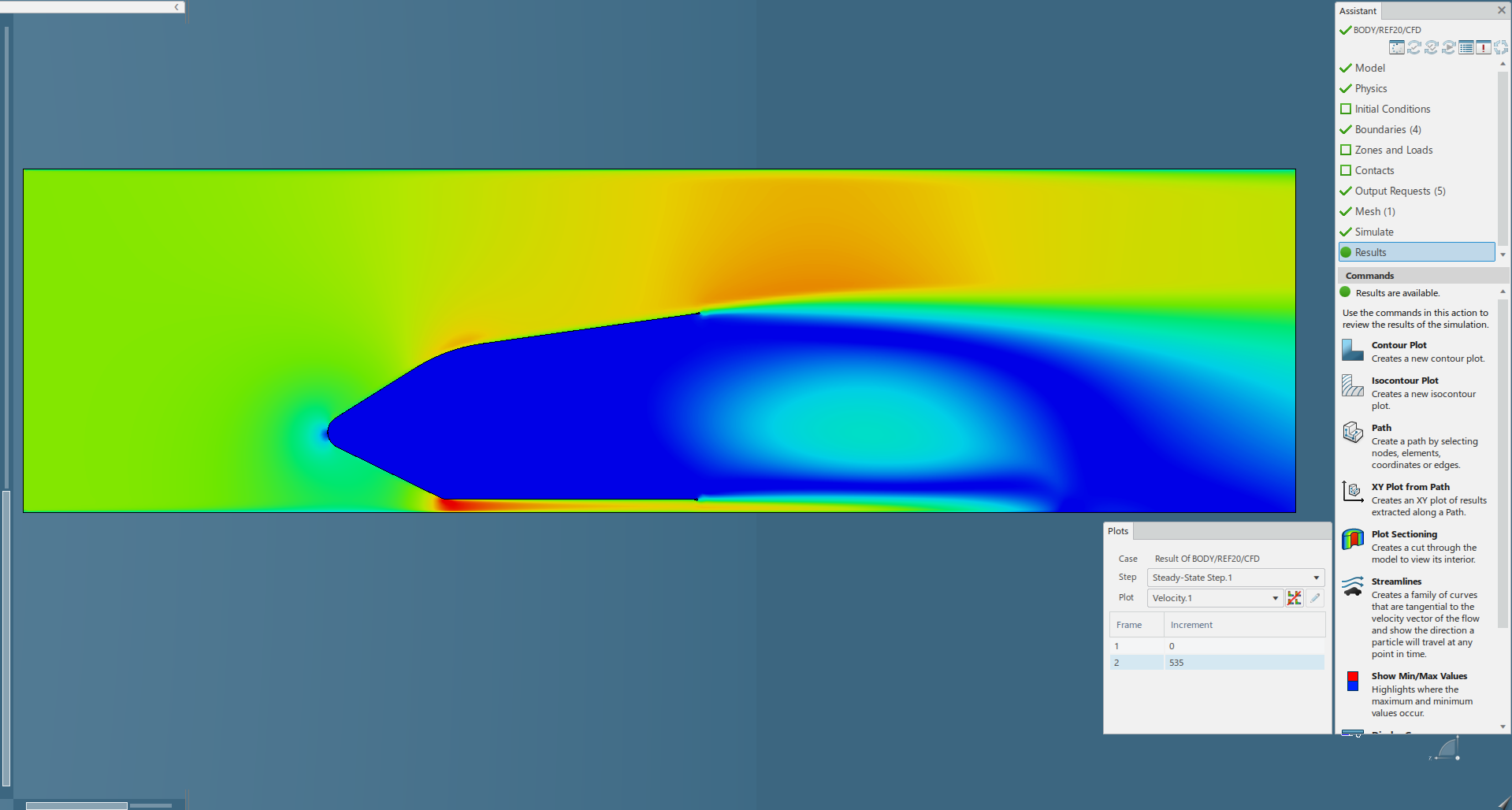
Figures 20. Velocity

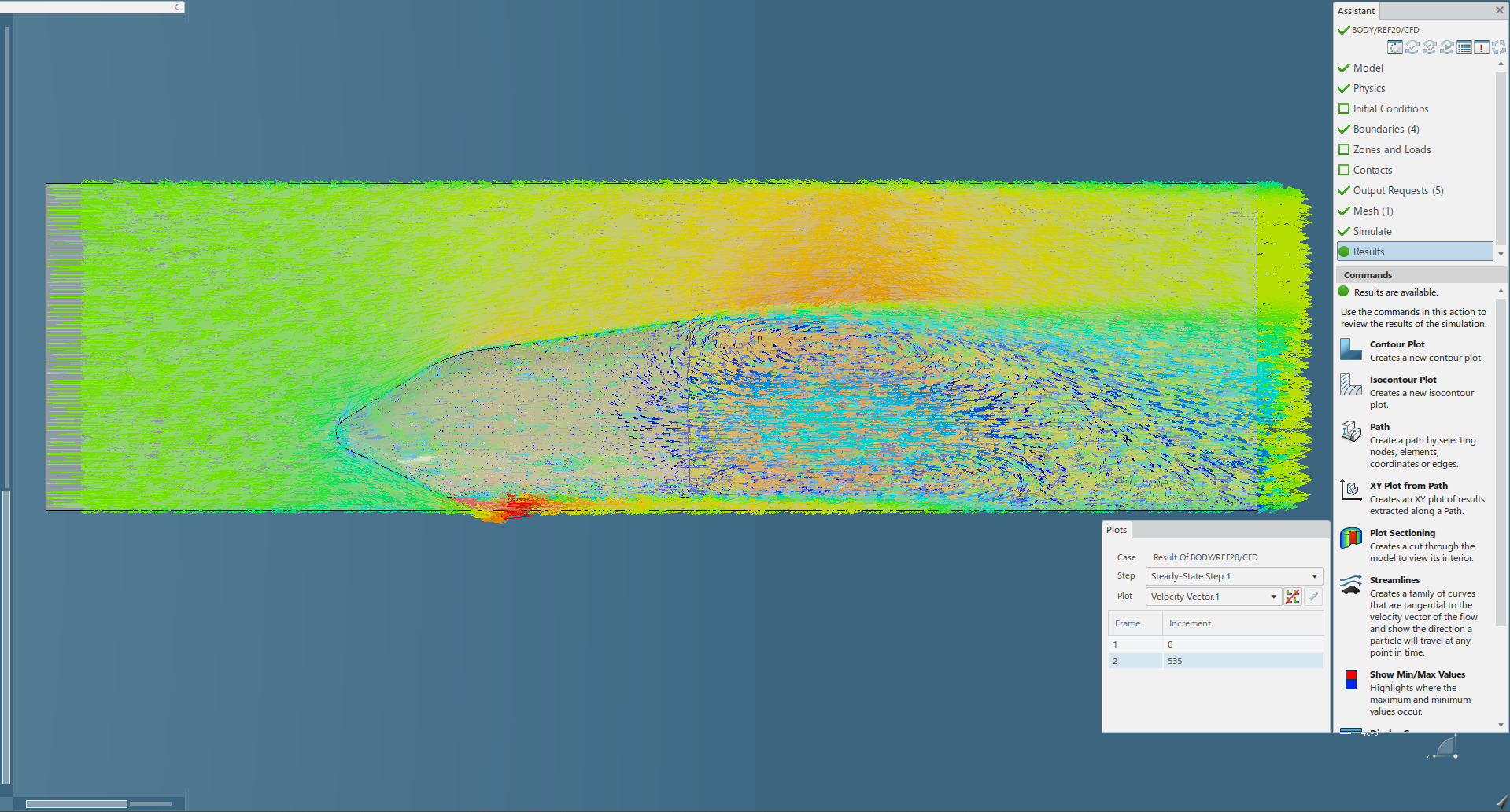
Figure 21. Velocity Vector

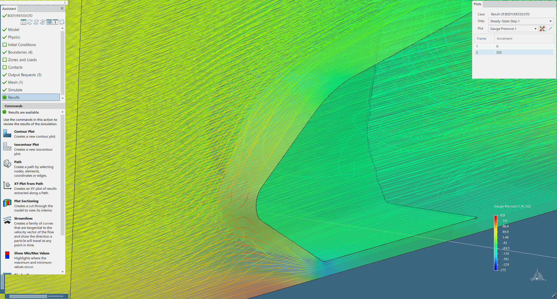
Figure 22. Gauge Pressure frame 2

Conclusion

Explaining this workflow was not as simple as I initially expected. The project combined two different areas: surface-quality evaluation in CATIA and aerodynamic analysis in SIMULIA.

While preparing this article, I realised that documenting each step also forced me to question my own decisions and better understand the reasoning behind every modelling choice.

The 3DEXPERIENCE community has been an important source of learning through shared projects, technical discussions and different engineering approaches.

I hope this article can also help other students who are starting to combine CATIA surface analysis with SIMULIA CFD and are looking for a practical example of a complete CAD-to-CFD workflow.

• Author
• Recent Posts

Abdulkadir Gunumdogdu

Vehicle Dynamics, Structural Analysis, Aerodynamics Design & CFD Engineer at Konrul Racing

Mechanical Engineering student and member of the Konrul Racing Team, focused on chassis design, CFD, structural analysis, and vehicle dynamics. Experienced with CATIA, 3DEXPERIENCE, and ANSYS for Formula Student and UAV development. Passionate about motorsport engineering and simulation-driven design.

Latest posts by Abdulkadir Gunumdogdu (see all)

• How to Set Up and Run a Formula Student CFD Simulation in SIMULIA (Part 2) - 10 August 2026
• How to Prepare a Formula Student Bodywork for CFD Using CATIA Surface Analysis (Part 1) - 29 July 2026